OLS Linear Regression: Hyperplane of Zero Net Force and Torque
Introduction
Linear regression is a commonly used technique. It was first used by Sir Francis Galton. Despite it’s dull nature, the term ‘regression’ has a significant implication as per Sir Galton’s study. Nowadays it is used in several applications to study the effect of change of one or more (independent) variables on a response variable.
In this article, I will attempt to look at linear regression through a different lens — physics. For simplicity, we will assume that all the assumptions of linear regression are satisfied.
The Mathematics
Linear regression has the form
\[y = \beta_0 + \beta_1*x_1 + \beta_2*x_2 + ... + \beta_n*x_n\]The conditional mean is estimated as
\[\hat{y} = b_0 + b_1*x_1 + b_2*x_2 + ... + b_n*x_n \tag{Equation 0}\]The ordinary least square solution is obtained by minimizing
\[\sum_{\forall i}(\hat{y}[i]-y[i])^2\]We apply calculus to the optimization problem by differentiating with respect to $b$ and setting the result equal to $0$. For each component $j$ we get:
\[\sum_{\forall i} (\hat{y}[i]-y[i])*x[i][j]=0 \tag{Equation 1}\]Substituting $j=0$ in the above equation for the intercept, we get:
\[\sum_{\forall i} \hat{y}[i]-y[i] = 0\]In addition we have the following property:
\[\sum_{\forall i} \bar{y}-y[i] = 0 \tag{Equation 2}\]Intuition

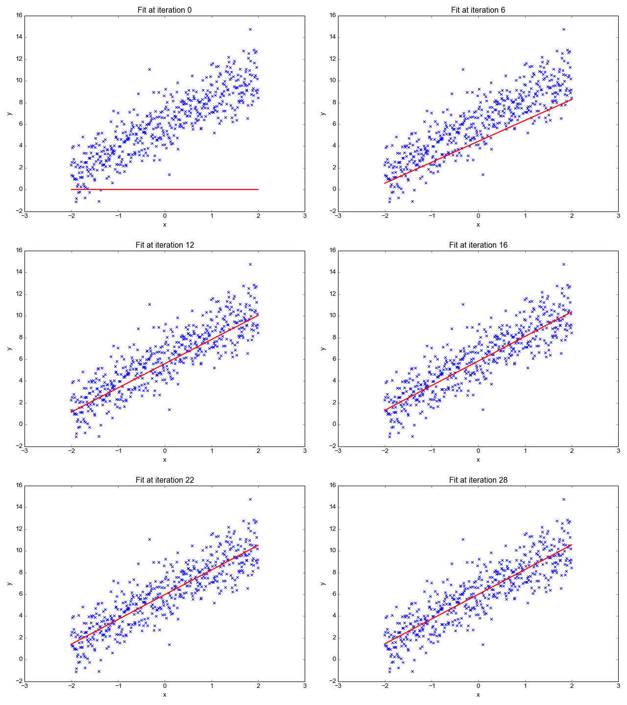
Image source: This post on Eli Bendersky’s website
Note: The above simulation is not a true representation of the process/logic described below because it does not ‘hinge’ on the point $(\bar{x}, \bar{y})$
Let’s take a step back and look at these results from a different lens. Let us consider aan ‘initial’ hyperplane that passes through $y=\bar{y}$ and has $b_1 = b_2 = … = b_n = 0$. We know that $\hat{y}[i] — y[i]$ is the prediction error for the $i^{th}$ training example after substituting in equation $0$. Let’s assume the error terms to be synonymous to force. Therefore, $error*x$ is synonymous to torque (this is a loose definition. To be more rigorous, the product should be defined more explicitly).
Based on equation $2$ we know that the net force on the ‘initial’ hyperplane is zero. However, the net torque is non-zero unless the OLS solution converges at $b_1 = b_2 = … = b_n = 0$. Let us imagine that the hyperplane is hinged on center of mass $(\bar{x}, \bar{y})$ and allowed to rotate freely by varying the slopes $b_1, b_2, …, b_n$. Each new orientation of the hyperplane will have zero net force because the errors cancel out. However, only 1 unique position of the hyperplane will have zero net torque. This is the solution to $argmin_{b} \sum_{\forall i} (\hat{y}[i] — y[i])^2 = argmin_{b} (\hat{Y} — Y)^T(\hat{Y} — Y)$ or $b = (X^TX)^{-1}X^TY$.
Under the standard assumptions of linear regression the OLS solution can be interpreted as a position of ‘stable equilibrium’. This interpretation of regression problems is just one of the paths to defining “generalization”.