CNN vs Fully-Connected Network for Image Processing
Introduction
The objective of this article is to provide a theoretical perspective to understand why (single layer) CNNs work better than fully-connected networks for image processing. Linear algebra (matrix multiplication, eigenvalues and/or PCA) and a property of sigmoid/tanh function will be used in an attempt to have a one-to-one (almost) comparison between a fully-connected network (logistic regression) and CNN. Finally, the tradeoff between filter size and the amount of information retained in the filtered image will be examined for the purpose of prediction. For simplicity, we will assume the following:
- The fully-connected network does not have a hidden layer (logistic regression)
- Original image was normalized to have pixel values between 0 and 1 or scaled to have mean = 0 and variance = 1
- Sigmoid/tanh activation is used between input and convolved image, although the argument works for other non-linear activation functions such as ReLU. ReLU is avoided because it breaks the rigor of the analysis if the images are scaled (mean = 0, variance = 1) instead of normalized
- Number of channels = depth of image = 1 for most of the article, model with higher number of channels will be discussed briefly
- The problem involves a classification task. Therefore, C > 1
- There are no non-linearities other than the activation and no non-differentiability (like pooling, strides other than 1, padding, etc.)
- Negative log likelihood loss function is used to train both networks
Symbols and Notation
Symbols used are:
- $x$: Matrix of 2-D input images
- $W_1$, $b_1$: Weight matrix and bias term used for mapping Raw image to output in fully-connected network Filtered image to output in CNN
- p: Output probability
- $X_1$: Filtered image
- $x_1$: Filtered-activated image
Two conventions to note about the notation are:
- Dimensions are written between {}
- Different dimensions are separated by x. Eg: {n x C} represents two dimensional ‘array’
Model definition
Fully-Connected Network
\[Z_{1[n \times C]}=x_{n\times(n_y*n_x)}WW_{1[(n_y*n_x)\times C]} + b_{1[1\times C]} \tag{FC1: pre-output layer}\] \[p_{[n\times C]} = F_{softmax}(Z_1)=\frac{[e^Z_1]_{[n\times C]}}{[\sum_{c=1}^{C} e_{C}^{Z_i}]_{n\times 1}} \tag{FC2: estimated probability}\]Convolution Neural Network
\[X_{1[n\times(y-k_y+1)\times(x-k_x+1)]}=x_{[n\times n_y \times n_x]}K_{[k_y\times k_x]} \tag{C1: filtered image}\] \[x_{1[n\times (n_y-k_y+1) \times (n_x-k_x+1)]} = \sigma(X_1) \tag{C2: filtered-activated image}\] \[\sigma^{(sigmoid)}(X_1)=\frac{e^{X_1}}{1+e^{X_1}}; \sigma^{(tanh)}(X_1)=\frac{e^{X_1}-e^{-X_1}}{e^{X_1}+e^{-X_1}} \tag{Activation functions}\] \[Z_{1[n\times C]}=x_{1[n\times (n_y-k_y+1) \times (n_x-k_x+1)]} \odot W_{1[(n_y-k_y+1) \times (n_x-k_x+1) \times C]} + b_{1[1\times C]} \tag{C3: pre-output layer}\] \[p_{n\times C} = F_{softmax}(Z_1) = \frac{e^{Z_1}}{1+e^{Z_1}} \tag{C4: estimated probability}\]The Mathematics
Reducing the CNN to a fully-connected network
Let us assume that the filter is square with $k_x = 1$ and $K(a, b) = 1$. Therefore, $XX_1 = x$. Now the advantage of normalizing x and a handy property of sigmoid/tanh will be used. It is discussed below:
Required property of sigmoid/tanh
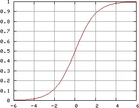
We observe that the function is linear for input is small in magnitude. Since the input image was normalized or scaled, all values x will lie in a small region around 0 such that $|x| < \epsilon$ for some non-zero $\epsilon$. Therefore, for some constant $k$ and for any point $X(a, b)$ on the image:
\[\sigma^{(sigmoid)}(X_1(a,b))_{[n\times 1]} \approx k*X_1(a,b)_{[n\times 1]}=k*x(a,b)_{[n\times 1]}\]This suggests that the amount of information in the filtered-activated image is very close to the amount of information in the original image. All the pixels of the filtered-activated image are connected to the output layer (fully-connected).
Let us assumed that we learnt optimal weights $W_1, b_1$ for a fully-connected network with the input layer fully connected to the output layer. We can directly obtain the weights for the given CNN as $W_1(CNN) = W_1/k$ rearranged into a matrix and $b_1(CNN) = b_1$. Therefore, for a square filter with $k_x = 1$ and $K(1, 1) = 1$ the fully-connected network and CNN will perform (almost) identically.
Since tanh is a rescaled sigmoid function, it can be argued that the same property applies to tanh. This can also be observed in the plot below:
Filter — worst-case scenario
Let us consider a square filter on a square image with $k_x = n_x$, and $K(a, b) = 1 \forall a, b$. Firstly, this filter maps each image to one value (filtered image), which is then mapped to $C$ outputs. Therefore, the filtered image contains less information (information bottleneck) than the output layer — any filtered image with less than $C$ pixels will be the bottleneck. Secondly, this filter maps each image into a single pixel equal to the sum of values of the image. This clearly contains very little information about the original image. Let us consider MNIST example to understand why: consider images with true labels ‘2’ and ‘5’. Sum of values of these images will not differ by much, yet the network should learn a clear boundary using this information.
Relaxing the worst-case part 1: filter weights
Let us consider a square filter on a square image with $k_x = n_x$ but not all values are equal in $K$. This allows variation in K such that importance is to give to certain pixels or regions (setting all other weights to constant and varying only these weights). By varying $K$ we may be able to discover regions of the image that help in separating the classes. For example — in MNIST, assuming hypothetically that all digits are centered and well-written as per a common template, this may create reasonable separation between the classes even though only 1 value is mapped to $C$ outputs. Consider this case to be similar to discriminant analysis, where a single value (discriminant function) can separate two or more classes.
Relaxing the worst-case part 2: filter width
Let us consider a square filter on a square image with K(a, b) = 1 for all a, b, but $k_x \neq n_x$. For example, let us consider $k_x = n_x-1$. The original and filtered image are shown below:
| $x_{1,1}$ | $x_{1,2}$ | $x_{1,3}$ | $x_{1,4}$ | … |
|---|---|---|---|---|
| $x_{2,1} $ | $x_{2,2}$ | $x_{2,3}$ | $x_{2,4}$ | … |
| $x_{3,1} $ | $x_{3,2}$ | $x_{3,3}$ | $x_{3,4}$ | … |
| … |
Table: Original image
\[(1,1): x_{1,1}+x_{1,2}+...+x_{1,n_x-1} + x_{2,1}+x_{2,2}+...+x_{2,n_x-1} + ... + x_{n_x-1,1}+x_{n_x-1,2}+...+x_{n_x-1,n_x-1}\] \[(1,2): x_{1,2}+x_{1,3}+...+x_{1,n_x} + x_{2,2}+x_{2,3}+...+x_{2,n_x} + ... + x_{n_x-1,2}+x_{n_x-1,3}+...+x_{n_x-1,n_x}\] \[(2,1): x_{2,1}+x_{2,2}+...+x_{2,n_x-1} + x_{3,1}+x_{3,2}+...+x_{3,n_x-1} + ... + x_{n_x,1}+x_{n_x,2}+...+x_{n_x,n_x-1}\] \[(2,2): x_{2,2}+x_{2,3}+...+x_{2,n_x} + x_{3,2}+x_{3,3}+...+x_{3,n_x} + ... + x_{n_x,2}+x_{n_x,3}+...+x_{n_x,n_x}\]Notice that the filtered image summations contain elements in the first row, first column, last row and last column only once. All other elements appear twice. Assuming the values in the filtered image are small because the original image was normalized or scaled, the activated filtered image can be approximated as $k$ times the filtered image for a small value $k$. Under linear operations such as matrix multiplication (with weight matrix), the amount of information in $k \times x_1$ is same as the amount of information in $x_1$ when $k$ is non-zero (true here since the slope of sigmoid/tanh is non-zero near the origin). Therefore, the filtered-activated image contains (approximately) the same amount of information as the filtered image (very loosely written for ease of understanding, because [Fisher] ‘information’ is the variance of the score function, which is related to the variance of the RV. A better version of this statement is: “the scaled/normalized input image and scaled/normalized filtered will have approximately the same amount of information”).
Assuming the original image has non-redundant pixels and non-redundant arrangement of pixels, the column space of the image reduced from $(n_x, n_x)$ to $(2, 2)$ on application of $(n_x-1, n_x-1)$ filter. This causes loss of information, but it is guaranteed to retain more information than $(n_x, n_x)$ filter for $K(a, b) = 1$. As the filter width decreases, the amount of information retained in the filtered (and therefore, filtered-activated) image increases. It reaches the maximum value for $k_x = 1$.
In a practical case such as MNIST, most of the pixels near the edges are redundant. Therefore, almost all the information can be retained by applying a filter of size ~ width of patch close to the edge with no digit information.
Putting things together
A peculiar property of CNN is that the same filter is applied at all regions of the image. This is called weight-sharing. The total number of parameters in the model is $(k_x \times k_y) + (n_x-k_y+1)\times (n_y-k_y+1)\times C$.
- Larger filter leads to smaller filtered-activated image, which leads to smaller amount of information passed through the fully-connected layer to the output layer. This leads to low signal-to-noise ratio, higher bias, but reduces the overfitting because the number of parameters in the fully-connected layer is reduced. This is a case of high bias, low variance.
- Smaller filter leads to larger filtered-activated image, which leads to larger amount of information passed through the fully-connected layer to the output layer. This leads to high signal-to-noise ratio, lower bias, but may cause overfitting because the number of parameters in the fully-connected layer is increased. This is a case of low bias, high variance.
It is known that $K(a, b) = 1$ and $k_x=1$ performs (almost) as well as a fully-connected network. By adjusting $K(a, b)$ for $k_x \neq 1$ through backpropagation (chain rule) and SGD, the model is guaranteed to perform better on the training set. It also tends to have a better bias-variance characteristic than a fully-connected network when trained with a different set of hyperparameters ($k_x$).
Summing up
A CNN with $k_x = 1$ and $K(1, 1) = 1$ can match the performance of a fully-connected network. The representation power of the filtered-activated image is least for $k_x = n_x$ and $K(a, b) = 1 \forall a, b$. Therefore, by tuning hyperparameter $k_x$ we can control the amount of information retained in the filtered-activated image. Also, by tuning $K$ to have values different from 1 we can focus on different sections of the image. By doing both — tuning hyperparameter $k_x$ and learning parameter $K$, a CNN is guaranteed to have better bias-variance characteristics with lower bound performance equal to the performance of a fully-connected network. This can be improved further by having multiple channels.
Extending the above discussion, it can be argued that a CNN will outperform a fully-connected network if they have same number of hidden layers with same/similar structure (number of neurons in each layer).
However, this comparison is like comparing apples with oranges. An appropriate comparison would be to compare a fully-connected neural network with a CNN with a single convolution + fully-connected layer. Comparing a fully-connected neural network with 1 hidden layer with a CNN with a single convolution + fully-connected layer is fairer.
MNIST data set in practice: a logistic regression model learns templates for each digit. This achieves good accuracy, but it is not good because the template may not generalize very well. A CNN with a fully connected network learns an appropriate kernel and the filtered image is less template-based. A fully-connected network with 1 hidden layer shows lesser signs of being template-based than a CNN.
References
1: https://www.researchgate.net/figure/Logistic-curve-From-formula-2-and-figure-1-we-can-see-that-regardless-of-regression_fig1_301570543
2: https://mathworld.wolfram.com/HyperbolicTangent.html