Lasso, Ridge and Dropout Regularization in Deep Learning — their effects on Collinearity
Introduction
This is a follow-up to my previous amateurish and rather cryptic article — A short note on regularization. The article delivered what it promised, but it is insufficient to answer the questions — what does regularization do and why does it work when the corresponding model without regularization doesn’t? The object of this article is to attempt to answer these questions using linear algebra (normal equations) and statistics (bias-variance tradeoff of estimators).
Let us assume that the engineered variables at a hidden layer of interest as $X$ or $x$, which is a function of the input features $Z$ or $z$. Throughout this article let us assume that intercept in 0 because in a general case the intercept is not shrunk. For simplicity, we will derive the analytical results for linear regression and generalize the results to logistic regression, assuming the true model is linear in the space of the (engineered) features.
Importance
I’m intentionally starting this article with the importance of regularization in machine learning. This section may be cryptic; the remainder of this article will build ideas from scratch in an attempt to understand these cryptic statements.
- Slicing a deep neural network along a fully-connected hidden layer with $h$ neurons leads to a smaller downstream neural network with $h$ features
- If the hidden layer chosen above is the layer before the output layer, the resulting neural network is equivalent to logistic regression
- Simple linear algebra that can be applied to linear/logistic regression can be extended to a deep neural network that is sliced at a fully-connected hidden layer
Linear Regression
Model Definition
\[Y=X\beta + \epsilon \tag{True model, unknown}\]Estimated Model
\[y=x\hat\beta^{(MLE)}+\hat{e}^{(MLE)} \tag{Estimated}\]Loss Function
\[L(\beta)=||y-x\beta||_2^2=(y-x\beta)^T(y-x\beta) \tag{Square loss in terms of matrix product}\]Solution
\[\hat{\beta}^{(MLE)}=argmin_\beta||y-x\beta||_2^2 \tag{ML/OLS estimate of coefficients}\]Reading: Equivalence of MLE and OLS in linear regression
Analytical Solution
\[\frac{\partial L}{\partial\beta}|_{\hat\beta^{(MLE)}}=0\implies -2x^T(y-x\hat\beta^{(MLE)})=0\implies \hat\beta^{(MLE)}=(x^Tx)^{-1}x^Ty \tag{Normal equations - MLE by analytical method}\]L2 Regularized Linear Regression
Model Definition
\[Y=X\beta + \epsilon \tag{True model, unknown}\]Estimated Model
\[y=x\hat\beta^{(Ridge)}+\hat{e}^{(Ridge)} \tag{Estimated}\]Loss Function
\[L(\beta)=||y-x\beta||_2^2 + \lambda||\beta||_2^2=(y-x\beta)^T(y-x\beta) + \lambda \beta^T\beta \tag{Loss in terms of matrix product}\]Solution
\[\hat{\beta}^{(Ridge)}=argmin_\beta||y-x\beta||_2^2 + \lambda||\beta||_2^2 \tag{Solution}\]Analytical Solution
\[\frac{\partial L}{\partial\beta}|_{\hat\beta^{(Ridge)}}=0\implies -2x^T(y-x\hat\beta^{(Ridge)})+2\lambda\hat\beta^{(Ridge)}=0\implies \hat\beta^{(Ridge)}=(x^Tx+\lambda I)^{-1}x^Ty \tag{Ridge estimate by analytical method}\]Understanding the difference
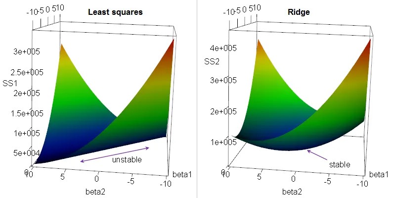
Consider a situation in which the design matrix is not full rank (few situations defined in my previous article: A short note on regularization). Therefore the covariance matrix is non-invertible. Therefore, the MLE does not exist.
Under this situation consider two extreme cases: $\lambda=0 \implies \hat\beta^{(Ridge)} = \hat\beta^{(MLE)}$ and $\lambda=\infty \implies \hat\beta^{(Ridge)}=0$. Between these 2 extreme cases, the modified covariance matrix given by $x^Tx+\lambda I$ will become diagonally dominant as $\lambda$ increases. Therefore, it is guaranteed to be invertible. This proves that the ridge estimate always exists (rigorous proof provided in this StackExchange article) for non-zero $\lambda$ even if the design matrix is not full rank.
Therefore, we conclude that the problem of collinearity is solved using L2 regularization. Lasso (L1 regularization) regression does not have an analytical solution unlike ridge regression. It is expected to behave similar to ridge regression in presence of collinearity. Lasso regression also performs pruning by shrinking the coefficient of variables to 0 as $\lambda < \infty$ increases, which is not observed in ridge (rigorous analysis of pruning by lasso can be found on my Quora answer). For convenience, L1 regularized linear regression formulation is presented below:
L1 Regularized Linear Regression
Model Definition
\[Y=X\beta + \epsilon \tag{True model, unknown}\]Estimated Model
\[y=x\hat\beta^{(Lasso)}+\hat{e}^{(Lasso)} \tag{Estimated}\]Loss Function
\[L(\beta)=||y-x\beta||_2^2+\lambda |\beta|_1=\sum_{i=1}^{p}(y-x_{(-i)}\beta_{(-i)}- x_{(i)}\beta_{(i)})^T(y-x_{(-i)}\beta_{(-i)}- x_{(i)}\beta_{(i)}) + \big[\lambda\sum_{j=1;j\neq i}^{p}|\beta|_j \big] + \lambda |\beta_i| \tag{Loss in terms of independent variables}\]Solution
\[\hat{\beta}^{(Ridge)}=argmin_\beta||y-x\beta||_2^2 + \lambda |\beta|_1 \tag{Solution}\]We assume that the behavior of lasso is similar to the behavior of ridge in terms of invertibility of the covariance matrix (a rigorous analysis can be found in this paper — page 5, also explains the reason for using coordinate descent). Analytical solution for lasso does not exist, except for a simple case — when the covariance matrix is a diagonal matrix.
Note on diagonal covariance: Parameter estimation becomes analogous to profile likelihood — change in a chosen $\beta$ in one iteration of coordinate descent does not affect other $\beta$s. Therefore, coordinate descent converges in 1 iteration.
Note: I will discuss L1 and L2 regularization in a more rigorous way with geometric interpretation in 2 separate articles.
Dropout
Dropout is often seen as a practical way of regularizing neural networks. It is difficult to treat dropout in an fully analytical way because:
- It involves some randomization — only the expected values are known, in practice individual realizations vary based on the seed
- It is performed on each sample/mini-batch/batch of (stochastic) gradient descent
The model can be viewed as:
\[M=X\odot R; R_{1\times h}~ Bernoulli(p) \tag{Masking variables in X at random; excluding intercept/bias}\] \[\hat{y}=f(x;\beta)=F_{sigmoid}(M\beta)\approx M\beta \tag{Linear regression on M vs y}\]Dropout has been used in practice to avoid correlation between weights. In practice this is done by randomizing the mask so that co-occurrence of variables is reduced. In theory the weights are correlated when the corresponding predictors are correlated. Therefore, masking using dropout helps in reducing overfitting.
Putting things together
Let us choose the hidden layer before the output layer. For $h « n$ (sample size) we observe that the problem of overfitting occurs when variables are collinear. L2 regularization explicitly removes the effect of collinearity by modifying the covariance matrix; L1 regularization affects the covariance matrix indirectly. Dropout affects the covariance between the weights by sampling from the set of features and masking the features that are not chosen (similar to random forest) during each update based on gradients.
Conclusion
Linear models and deep neural networks are related through linear algebra. Over determined systems (number of predictors > number of samples) and collinear systems (rank < number of predictors) lead to unstable solutions and overfitting that can be resolved using regularization. The 3 most common forms of regularization — ridge, lasso and droupout — reduce overfitting by reducing the collinearity among predictors (or hidden layer in deep neural networks). But it is important to note that collinearity is not the only cause of overfitting. There are other forms of regularization that penalize the curvature in each dimension (check smoothing splines).
A more rigorous analysis with geometric interpretation of ridge and lasso will be published in the future.
Further reading
Research paper: Reducing overfitting in deep neural networks by decorrelating representations
Research paper: Regularizing deep neural networks with an ensemble-based decorrelation method
Related research paper: A weight set decorrelating training algorithm for neural network interpretation and symmetry breaking
Related research paper: A decorrelation approach for pruning of multilayer perceptron networks