Lasso Regularization on Linear Regression and Deep Learning Models
Introduction
Curve fitting — under and over fitting
As discussed in my previous article, issues with ‘curve fitting’ occur when the problem is ill-posed. Underfitting is usually not a big problem because we have the option to expand the feature set by acquiring/engineering new features. However, overfitting is not easy to handle.
Best subset selection in regression
Consider a linear regression with $p$ predictor variables. Assume that the whole data set is used for training. It is known that the training set $R^2$ never decreases on addition of features. Therefore, $R^2$ is not always a good measure of goodness of fit. Adjusted-$R^2$, Mallow’s $C_p$, AIC, BIC, etc. are used to measure the goodness of fit. However, a priori knowledge does not exist on the change in values of these measures upon addition/removal of predictor variables. Therefore, all $2^p-1$ distinct models may be required to judge the ‘best subset’ of features required to model the outcome variable. However, this is computationally very expensive. This necessitates an appropriate way to reduce variables without building exponentially large number of models. Lasso penalty helps in achieving this goal partially.
Formulation
Linear regression and normal equation
\[Y=X\beta + \epsilon \tag{Regression equation}\] \[y=x\hat\beta^{(MLE)}+\hat{e}^{(MLE)} \tag{Linear regression estimated on a sample}\] \[L(\beta)=||y-x\beta||_2^2 \implies \hat\beta^{(MLE)}=argmin_\beta ||y-x\beta||_2^2 \tag{OLS solution — same as MLE under certain conditions}\] \[\frac{\partial L}{\partial\beta}|_{\hat{\beta}^{(MLE)}}=0 \implies x^T(y-x\hat\beta^{(MLE)})=0 \implies \hat\beta^{(MLE)}=(x^Tx)^{-1}x^Ty \tag{Normal equations}\]We observe that the OLS solution does not exist (may not be unique) if the covariance matrix is non-invertible.
Lasso formulation
\[Y=X\beta + \epsilon \tag{Regression equation}\] \[y=x\hat\beta^{(Lasso)}+\hat{e}^{(Lasso)} \tag{Lasso solution estimated on sample}\] \[L(\beta)=||y-x\beta||_2^2 + \lambda |\beta|_1 \implies \hat\beta^{(Lasso)}=argmin_\beta \big[||y-x\beta||_2^2 + \lambda |\beta|_1\big] \tag{Lasso solution}\]Analytical solution does not exist for this minimization. Also gradient descent is not guaranteed to converge on this loss function even though it is convex. An alternate formulation is required to computationally solve this problem.
Solution
Soft thresholding for orthogonal covariance
\[L(\beta)=||y-x\hat\beta^{(OLS)}+x\hat\beta^{(OLS)}-x\beta||_2^2+\lambda|\beta|_1\] \[L(\beta)=||y-x\hat\beta^{(OLS)}||_2^2 - 2(y-x\hat\beta^{(OLS)})^T x(\hat\beta^{(OLS)}-\beta) + ||x\hat\beta^{(OLS)}-x\beta||_2^2+\lambda|\beta|_1; y-x\hat\beta^{(OLS)} = \hat{e}^{(OLS)} \perp x\] \[\implies \hat\beta^{(Lasso)}=argmin_\beta \big[X(\hat\beta^{(OLS)}-\beta)\big]^T \big[X(\hat\beta^{(OLS)}-\beta)\big] + \lambda |\beta|_1\] \[\implies \hat\beta^{(Lasso)}=argmin_\beta (\hat\beta^{(OLS)}-\beta)^TX^T X(\hat\beta^{(OLS)}-\beta) + \lambda |\beta|_1\]Assuming $X^T X=I$
\[\hat\beta^{(Lasso)}=argmin_\beta (\hat\beta^{(OLS)}-\beta)^T(\hat\beta^{(OLS)}-\beta) + \lambda |\beta|_1\] \[\implies \hat\beta^{(Lasso)}=argmin_\beta (\hat\beta^{(OLS)}_i-\beta_i)^2 + \lambda |\beta_i|_1 + \sum_{j=1;j\neq i}^{p}\big[(\hat\beta^{(OLS)}_j-\beta_j)^2 +\lambda |\beta_j|_1\big]\] \[\implies \hat\beta_i^{(Lasso)} = argmin_{\beta_i} \big[(\hat\beta^{(OLS)}_i-\beta_i)^2 +\lambda |\beta_i|_1\big] \tag{Separating out the dimensions}\] \[\hat\beta_i^{(Lasso)}= \begin{cases} \hat\beta_i^{(OLS)}-\frac{\lambda}{2}& \text{if } \hat\beta_i^{(OLS)}>\frac{\lambda}{2}\\ 0 & \text{if }|\beta_i^{(OLS)}| \le \frac{\lambda}{2}\\ \hat\beta_i^{(OLS)}+\frac{\lambda}{2}& \text{if } \hat\beta_i^{(OLS)}<-\frac{\lambda}{2} \end{cases} \tag{Soft thresholding}\]Soft thresholding can be performed on each dimension individually. This update will converge to the optimal $\beta$ since they are independent. This idea is similar to profile likelihood — estimation of a critical parameter is done by profiling out (fixing) noisy parameters and maximizing the likelihood (assumed convex), then the noisy parameters are estimated by fixing the critical parameter at its computed optimum value: this works when the parameters are independent.
This method of updating one parameter at a time is called coordinate descent.
Coordinate descent: general case
For a general case without orthogonal design coordinate descent can be summarized as follows:
vector coordinateDescent(int p, int max_iter, double epsilon) {
  Randomly initialize vector beta(p);
  ...
  for(i = 0; i < max_iter; i++) {
    for(j = 0; j < p; j++) {
      Calculate residuals by setting beta[j]=0;
      Regress residual on j-th predictor, obtain OLS solution for beta[j];
      Apply soft-thresholding on beta[j];
      Check for convergence: first norm of update in beta < epsilon;
    }
  }
  ...
  return(beta);
}
The full code with an example can be found here.
Coordinate descent is guaranteed to converge in one iteration (the second iteration will not update the weights) for orthogonal design. It is not guaranteed to converge in 1 iteration if the design matrix is not orthogonal, but it will converge in finite number of iterations.
Geometric Interpretation
Dual form of optimization
\[Loss = ||y-x\beta||_2^2+\lambda |\beta|_1 \tag{Lasso loss}\] \[min(Loss) \sim min(||y-x\beta||_2^2);\text{ s.t. }|\beta|_1 \le s; s=f(\lambda) \tag{Dual form of Lasso optimization}\]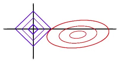
The blue squares correspond to $|\beta|_1 \le s$ for different $s$, where $|\beta|_1 = constant$ along a square. Increasing $\lambda$ decreases the size of the square. The red ellipses correspond to different distinct values of $||y-x\beta||_2^2$ where $||y-x\beta||_2^2=constant$ along an ellipse. For a fixed $\lambda$ the value of $s$ is fixed: this corresponds to one of the blue squares.
The minimum value of $||y-x\beta||_2^2$ in unconstrained case occurs at the center of the ellipse. However, under the constrained case of $|\beta|_1 \le s$ the solution will be displaced towards the origin.
The unique lasso solution is located at the point where these two ‘curves’ touch. Since the curve $|\beta|_1 \le s$ is non-differentiable at few points the lasso solution for few $\beta_i$s can be zero. On increasing $\lambda$ (decreasing $s$) these $β_i$s remain 0; other $β_i$s tend to 0. This causes sparsity in the coefficients of lasso.
Extension to deep learning
Deep learning networks inevitably have fully-connected layers. These layers perform linear transformation on the input and apply an activation on the transformed variables. When the transformed outputs are small in magnitude (typically less than 1) the non-linearity can be ignored. With lasso penalty on the weights the estimation can be viewed in the same way as a linear regression with lasso penalty. The geometric interpretation suggests that for $\lambda > \lambda_1$ (minimum $\lambda$ for which only one $\beta_j=0$) we will have at least one weight = 0. This creates sparsity in the weights. This argument also applies to non-linear cases with large values of transformed inputs.
Conclusion
Lasso penalty creates sparsity in coefficients by driving some of the coefficient to 0. This applies to linear regression and fully-connected layers in deep neural networks. Therefore lasso penalty can reduce the complexity of deep learning models for suitable values of $\lambda$. However, it is not a solution for all problems.
If the underlying model is linear ($Y = X\beta + \epsilon$), non-zero $\lambda$ leads to bias in the lasso solution ($E(\hat\beta^{(Lasso)}) \neq \beta$ but the estimator has lower variance than MLE) — therefore it cannot achieve estimation and selection consistency simultaneously even for simple cases. Despite this shortcoming it is a good solution to overfitting on finite samples, especially in deep neural networks with large number of parameters that tend to overfit.