Understanding the Expressive Power of ReLU Networks
Introduction
This article was inspired by Wilson Wang’s article - Understanding the Expressive Power of Neural Networks. Wilson’s original article is applicable to a wide range of activation functions.
The focus of this article is to create a spline equivalent of a single hidden layer neural network that uses ReLU activation for a regression model and to quantify degrees of freedom (proxy for bias-variance tradeoff) of the corresponding spline - therefore the degrees of freedom of the neural network (not something most people are familiar with). For simplicity, we will use a one-dimensional input feature vector $X$, output feature vector $y$ and OLS loss without regularization.
While most of these ideas can be derived using a simple graph and intuition alone, this article will build everything from scratch and attempt to leave no ends untied.
Part 1: Splines
Splines can be considered as extensions to polynomial curve fitting by incorporating ‘kinks’ (aka knots) in the curves that are placed at appropriate locations. These kinks may or may not be points of discontinuities or non-differentiabilities. In this section we will focus on different levels of ‘flexibility’ and ‘robustness’ (often competing forces in the bias-variance tradeoff) of splines.
Histogram regression
Consider a discretization of the input feature (for example: equal or unequal interval binning). Formally, we can define the basis as:
\[I(X_l^{(i)}<X<X_u^{(i)}); i \in \{1, 2, ..., i_{max}\}; (X_l^{(1)}, X_u^{(i_{max})})=(-\infty, \infty); X_u^{(i-1)}=X_l^{(i)} \tag{Basis vector of histogram regression spanning the whole range of x}\]Let the updated feature matrix with the binary features stacked as columns be $M$. We have the histogram regression model defined as:
\[Y=M\beta + \epsilon \tag{Histogram regression model}\] \[y=M\hat{\beta} + \hat{e} \tag{Histogram regression sample estimates}\]Degrees of freedom of the model is given by $min(i_{max}+1, N_{train})$.
Piecewise linear with discontinuities
Similar to the discrete piecewise binary basis of a histogram regression model, consider a piecewise linear basis defined as:
\[I(X_l^{(i)}<X)X; i \in \{1, 2, ..., i_{max}\}; (X_l^{(1)}, X_u^{(i_{max})})=(-\infty, \infty); X_u^{(i-1)}=X_l^{(i)} \tag{Basis vector of piecewise linear regression (with discontinuities) spanning the whole range of x}\]The definition the model does not change — it is linear with respect to the parameters and with respect to the independent variables. We have the histogram regression model defined as:
\[Y=M\beta + \epsilon \tag{Piecewise linear model with discontinuities}\] \[y=M\hat\beta + \hat{e} \tag{Piecewise linear model with discontinuities — sample estimates}\]Since $k$ knots will divide the real number line into $k+1$ segments identified by the order statistics of the knots, and each region has a slope and an intercept, the degrees of freedom of the model can be written as $min(2*i_{max}+1, N_{train})$.
Piecewise linear continuous
Similar to the basis of a piecewise linear model with discontinuities, consider a new piecewise linear basis defined as:
\[1, X, \left\{I(X_l^{(i)}<X)(X-X_l^{(i)}); i \in \{1, 2, ..., i_{max}\}\right\}; X_l^{(1)}>-\infty; X_u^{i_{max}}<\infty; X_u^{(i-1)}=X_l^{(i)} \tag{Basis vector of piecewise linear regression (continuous) spanning the whole range of x}\]The definition of the model and estimates take the same form as the previous two models and estimates respectively. The interesting aspect of this model is that it is less expressive than a piecewise linear model with discontinuities because of the continuity constraints at the knots. Therefore, we compute the degrees of freedom of the model as $min(i_{max}+2, N_{train})$.
Note 1: Fitting a model after fixing the number of knots
Usually the choice of knots for a given training set is such that $i_{max} < N_{train}$. The search for the best ‘knots’ for a piecewise fit is a computationally complex problem even for relatively small values of $i_{max}$ and $N_{train}$. If all the samples of $x$ are distinct, and if we assume all the knots coincide with a training example, a brute force search requires ${N_{train} \choose i_{max}}$ [upper bounded by $O(2^{N_{train}})$] computations to find the best solution. Neat tricks exist for well behaved data sets - discussed here
Note 2: Identifying the best number of knots
Cross validation can be used to determine the best number and position of knots. The model is underdetermined (overfit) if the number of mutually exclusive and independent discretizations is close to 0. For example, for the extreme case of a single discretization (no knots, intercept only), the model exhibits high bias and low variance. The model is overdetermined (overfit) if the number of mutually exclusive and independent discretizations is larger than the number of training examples. For example, for the extreme case of a knots between each data point (knots = {sample order statistics}), the model exhibits low bias and high variance.
Part 2: ReLU activation in neural networks
In this section we will discuss how ReLU activation at the hidden layers and linear activation at the output layer equates to a piecewise linear model. For this purpose we will assume at least one hidden layer; ReLU activation will be applied at each hidden layer.
Single hidden layer
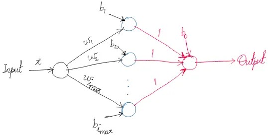
Output as a function of the input is $Output=b_0+ReLU(w_1x+b_1)+ReLU(w_2x+b_2)+…+ReLU(w_{i_{max}}x+b_{i_{max}})$. Slope of the ‘line’ changes at the points $x = (-b_1/w_1), (-b_2/w_2), …, (-b_{i_{max}}/w_{i_{max}})$ Therefore, these points act as knots. Let’s sketch the output as a function of the input for two knots:
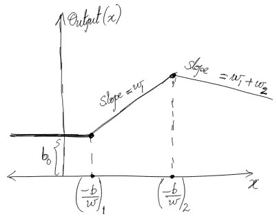
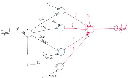
The missing piece from a piecewise continuous model is an additional slope for $x$ smaller than the first knot point (first order statistic of $-b/w$). This can be accomplished by forcing a knot at $-\infty$ (extra neuron in the hidden layer with bias constrained at $-\infty$) or by adding a weighted residual connection at the output.
Putting the pieces together
Equivalence of the functions
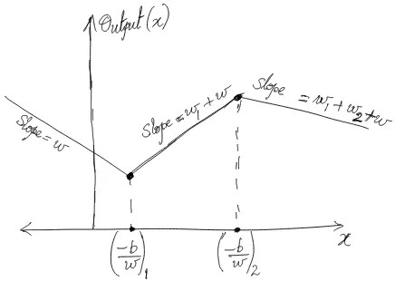
Looking at the final diagram for a ReLU network, we can conclude that the output is a piecewise linear function of the input. Let us assume that the order statistics of $-b/w$ magically coincide with the order statistics of the knots of a piecewise continuous linear model. The question is - if the global minimum solutions are considered for the OLS loss, are these two models equivalent? The answer looks like an obvious yes if the solution is unique (expected to be the case because the knots in both models are distinct and number of training examples > number of knots), but a rigorous proof requires a check for consistency of the system of equations:
\[w^{ReLU}=w_x^{Spline}\] \[b_0^{ReLU}=b^{Spline}\] \[(w_1+w)^{ReLU}=(w_{I(X_l^{(1)} < X)}+w_x)^{Spline}\] \[(w_2+w_1+w)^{ReLU}=(w_{I(X_l^{(2)} < X)} + w_{I(X_l^{(1)} < X)}+w_x)^{Spline}\]We observe that for the basis definition that was used for the piecewise linear model and ReLU neural network, the weights equate exactly.
Conclusion
A ReLU neural network with a single hidden layer is a scaled piecewise linear model with the same number of knots as the number of neurons. Therefore, the degrees of freedom of the (updated) ReLU neural network is $min(i_{max}+2, N_{train})$
The two additional degrees of freedom give the network flexibility to extrapolate beyond the range of the training set. The system is overdetermined if the number of knots > number of training examples.
Extended discussion
- Reiterating: a. Choosing the best knots is computationally complex b. Since ReLU neural networks have to accomplish a complex search task by adjusting $(b,w)$, they may get stuck in local optima. The observations of this paper and this paper should be intuitive and unsurprising, but the underlying math is not! c. Cross validation can be used for choosing the best number of knots
- What happens when we add more hidden layers with ReLU activation? More knots are added
- Where does this take us? Clearly adding too many knots leads to overfitting. More complex basis functions can be a better alternative
- What about regularization? Regularization extends the idea of nonlinear basis in splines to build smoothing splines for automatically selecting knots that are ideal for the data set
- Extension to multivariate settings $w^1_x x+w^1_y y+b^1=0$ is the equation of a line in the xy plane. Therefore, the ‘knots’ will be hyperplanes a. An important talk on interpolation of ReLU networks: https://www.youtube.com/watch?v=86ib0sfdFtw b. With the limited background provided by this article, the observations of this paper and this paper should be understandable