‘Manufacturing’ polynomials using a sigmoid neural network

Introduction

The objective of this article is to understand how (deep) neural networks with sigmoid activation can manufacture polynomial-like functions. The objective of this article is to only “engineer” possible bases (plural of basis in linear algebra) for higher order polynomials in the hidden layers to approximate any polynomial function using a sigmoid neural network with appropriate depth and width. It is important to highlight that the objective of this article is not to engineer the most optimal bases in the hidden layer.

For simplicity, we will assume a regression problem with OLS loss (without regularization) that relates the output variable y to a single input variable $x$. Also, we will assume that $x$ is standardized to have 0 mean and unit variance, the output layer uses a linear activation, and all the hidden layers use a sigmoid activation.

As usual, my objective is to answer a few fundamental “why” questions in deep learning. Unlike my usual articles, this article will rely more on visuals and intuition over more rigorous mathematical ideas and proofs. However, this article will be child’s play for seasoned deep learning experts who know how things work.

Part -1: the sigmoid activation function

\[\sigma(x) = Sigmoid(x) = \frac{1}{1+e^{-x}} = \frac{e^x}{1+e^x}\] \[\sigma'(x) = \frac{\partial \frac{1}{1+e^{-x}}}{\partial x} = -\frac{1}{(1+e^{-x})^2}(-e^{-x}) = e^{-x}\sigma(x)^2 \ge 0 \forall x \in (-\infty, \infty)\]

Part 0: the constant term

We all know the sigmoid function well. It is asymptotic at both extremes — which means its value is almost constant as $|x|$ tends to large values. If we define a region $S_0$ such that $|\sigma(x)-c_0|<\epsilon_0 \forall x ∈ S_0$. Roughly we can assume $S_0=(-\infty, -6) \cup (6, \infty)$

Part 1: the linear term

$\sigma(x) = Sigmoid(x)$ vs $x$ for $x \in (-10, 10)$

I’m not going to explain the omnipresent sigmoid in this article. From the plot we infer that the $\sigma(x)$ looks linear (loosely speaking) with respect to $x$ for $x \in (-1, 1)$. But is it really?

For a more rigorous proof: Assume $y_1(w_1x)=a_1w_1x+b_1$ is the linear representation of $\sigma(x)$ around $L_1$ (it should be immediately clear that $b_1=0.5$). Then $y_1(x)$ should be such that there exist $(a_1, \epsilon_1>0, \delta_1>0)$ that satisfy:$|y_1(x)-\sigma(x)| < \epsilon_1 \forall x \in (L_1-\delta_1, L_1+\delta_1)$

Alternatively, let us examine the first derivative — if the first derivative is ‘almost constant’ in a region $S_1$ disjoint from $S_0$, then the original function is ‘almost linear’ in that region.

$\sigma'(x)$ vs $x$ for $x \in (-10, 10)$

Using $\sigma’(x)\ge 0.19$ (margin of error ~ 24%) we get something close to our previous guess - $L_1=0, a_1/w_1 \in (0.19, 0.25), \delta_1 \sim 1 \implies S_1 = (-1, 1)$ works reasonably well to manufacture the linear term.

Part 2: the quadratic term

For a more rigorous proof: Assume $y_2(w_2x)=a_2(w_2x)^2+b_2(w_2x)+c_2$ is the quadratic representation of $\sigma(x)$ around $L_2$. Then $y_2(x)$ should be such that there exist $(a_2, \epsilon_2>0, \delta_2>0)$ that satisfy:$|y_2(x)-\sigma(x)| < \epsilon_2 \forall x \in (L_2-\delta_2, L_2+\delta_2)$

Instead, let us examine the second derivative — if the second derivative is ‘almost constant’ in a region $S_2$ disjoint from $S_1$ and $S_0$, then the original function is ‘almost quadratic’ in that region.

From the graph let us choose $\sigma’‘(x)\ge0.091$ (margin of error ~ 9%, this is not a fluke or a guess, it involved some trial and error). Solving using Wolfram Alpha (link to the solution I used), $a_2/w_2^2\sim 0.0455$, $S_2 = (-1.67, -1) \cup (1, 1.67)$ works reasonably well to manufacture the quadratic term.

Part 3: the cubic term and other higher order terms

We need to find $y_3(w_3x)=a_3(w_3x)^3+b_3(w_3x)^2+c_3(w_3x)+d_3$ that approximates $\sigma(x)$ in some region $S_3$. We already used the region $S_1=(-1, 1)$ to manufacture the linear term. From the graph let us choose $\sigma’’‘(x)\ge 0.035$ (margin of error ~ 16%). Solving using Wolfram Alpha (link to the solution I used), $a_3/w_3^3 \sim 0.0058$, $S_3 = (-2.89, -1.86) \cup (1.86, 2.89)$ works reasonably well to manufacture the cubic term.

Similarly, higher order polynomial terms can be manufactured from appropriate regions of the sigmoid curve.

$\sigma^{iv}(x)$ vs $x$ for $x \in (-10, 10)$

$\sigma^{v}(x)$ vs $x$ for $x \in (-10, 10)$

Putting things together: a wide single hidden layer neural network

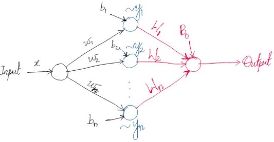
Neural network to manufacture an n-th order polynomial

We take a leap of faith — we assume that for any arbitrary choice of $n$ we will be able to find a non-null $S_n$ that is disjoint from $S_0, S_1, S_2, …, S_{n-1}$. This should be mathematically feasible because the Taylor series expansion of $\sigma(x)$ exists around any value of x, and at least some of the higher order terms will be non-zero.

Remember, $x$ was centered and scaled, therefore $w*x$ is bounded. For appropriate choices of $b$ we can map $x$ to the appropriate polynomial region. The output is a weighted sum of polynomials of order less than or equal to $n$. Therefore, the output is a polynomial of order $n$.

Closing notes

For a chosen order of polynomial it should be noted that the weights are constrained by the range of $S$. The coefficient of the n-th order polynomial $y$ (given by $max(\sigma^{n’}(x))/n!$) decreases as $n$ increases
Any polynomial can be approximated by adjusting the weights. $W$’s should be of greater interest for the purpose of updating the parameters, and $w$’s should be considered as restricted parameters used for engineering features
$\frac{a_1}{w_1}\frac{a_2}{w_2^2} \sim 0.19*0.0455 = 0.0086 > \frac{a_3}{w_3^3} \sim 0.0058$ [we still haven’t figured out how to engineer interaction terms as features, so let’s ignore this for now]; $(\frac{a_2}{w_2^2})^2 \sim 0.002 > \frac{a_4}{w_4^4} \sim 0.0008$. Therefore, a deeper network is better for more readily engineering higher order polynomials. This can be attributed to the increase in number of parameters of the network

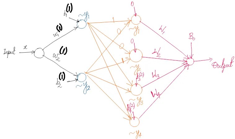
‘Deep’ neural network for higher order polynomials (notice that some biases and weights are fixed/frozen/not updated for ease of interpretation)

Also, it is known that building up non-linear features gradually in the deeper layers is often a better strategy than forcefully engineering them in the first hidden layer by having a very wide network - this also helps in robustness. However, for a given ‘$n$’ we have not established whether indefinitely increasing the depth of the neural network (to $\infty$) is the best approach, or if there is an optimal number of hidden layers. In addition, we have not proved that this approach is the most optimal way to generate an n-th order polynomial using a sigmoid neural network. Note that these proofs require us to optimally choose the number of neurons in each layer. However, this should remind us of a familiar heuristics - number of neurons ~ squared after each layer or expanding out in powers of 2 in the deeper layers.

Understanding the Expressive Power of ReLU Networks

‘Manufacturing’ polynomials using a sigmoid neural network - practicum