‘Manufacturing’ polynomials using a sigmoid neural network - practicum
Introduction
In the previous article I discussed a possible way to create polynomial bases (plural of basis in linear algebra) to approximate a polynomial function using a sigmoid neural network. This article is a practical test of the idea - does the bias constraint work as predicted, and how does it compare with a sigmoid neural network without the bias constraint? We will assume a quadratic true model of the form $y = ax^2+bx+c+\epsilon$; for convenience, $\epsilon=0, c=1, b=2, a=3$.
The code
Repository: https://github.com/SNaveenMathew/ml_book/tree/master/polynomial_regression
Files (in the required order):
Bias constrained sigmoid neural network
Model definition
Bias constraints
$b_1=0, b_2=log(2-\sqrt{3}) \sim -1.317$ — these parameters were not updated during training, whereas $(w_1, w_2, W_1, W_2, B_0)$ are unconstrained.
Training
A data set was generated using 10000 observations from $x\sim N(0, 1); y = 3x^2+ 2x+1$ (training set generation and true model are defined in quadratic_model.py). Since the objective is not to perform model selection or hyperparameter tuning, all 10000 observations were used for training.
Weights
The model was trained for a very large number of epochs. The final model parameters were:
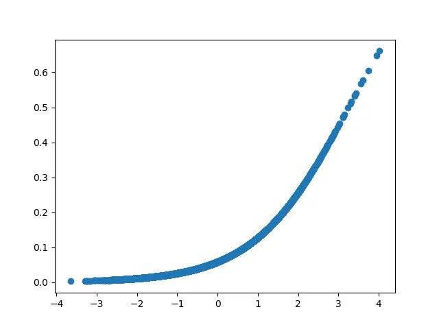
\[(w_1, w_2, W_1, W_2, B_0) = (0.192, 0.396, -549.653, 427.676, 185.346); loss \sim 0.0458\]Visualizing $y_1, y_2$ vs $x$
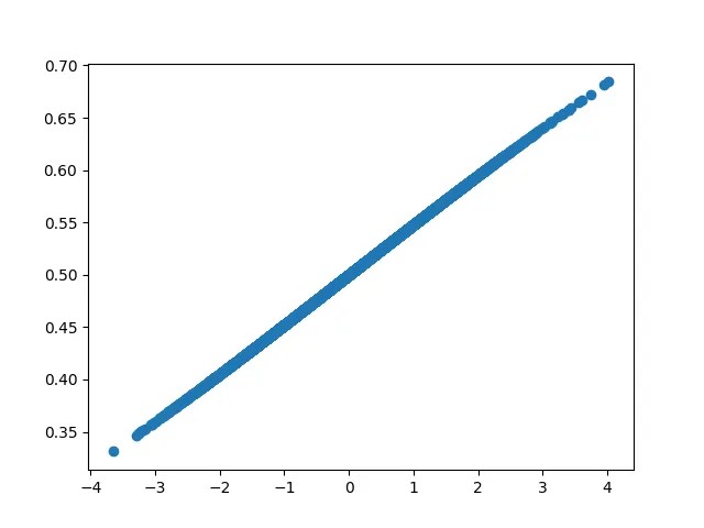
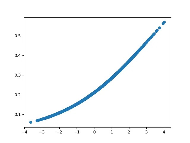
From the visual representation we can vaguely infer that the model is learning exactly what we expect it to learn — $y_1$ learns the linear part, $y_2$ learns the quadratic part. But is this inference accurate?
Deep dive
$y_1$

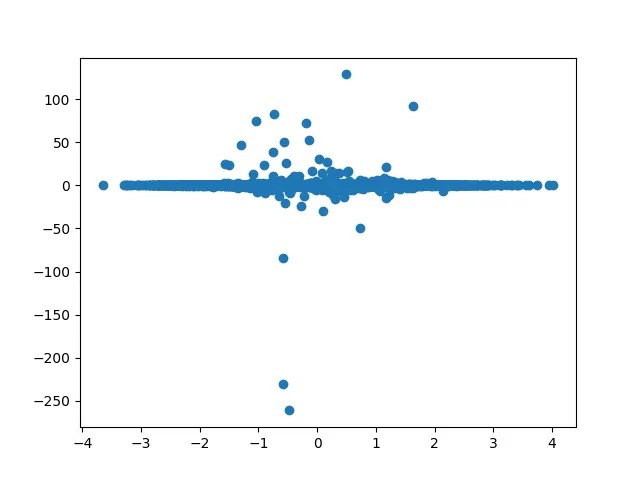
$\frac{\partial y_1}{\partial x}$ was computed by sorting $x$ and computing the forward difference approximation using $\frac{\delta y_1}{\delta x}$ by considering the discrete points of $x$ in the training set. We observe that $f_1$ is almost linear with respect to $x$, but shows some signatures of higher order polynomial terms. The estimate for $\frac{\partial y_1}{\partial x}$ is 0.04784 (sample median). Using this the theoretical approximation for the coefficient of the linear term is 0.04784.
$y_2$
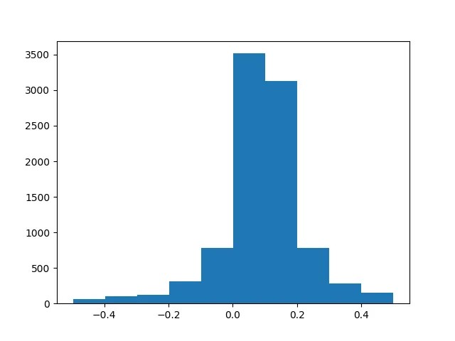
We observe that $\frac{\partial^2y_2}{\partial x^2}$ is almost a constant. The estimate for $\frac{\partial^2y_2}{\partial x^2}$ is 0.0973 (sample median). Using this the theoretical approximation for the coefficient of the quadratic term is 0.0486. The estimate differs from the theoretical value of 0.0455.
Final polynomial function approximation
Fitting a linear model to the outcome, we obtain the MLE for the equation $y = w_1y_1+w_2y_2+w_3+\epsilon_3$ as $w_1\sim -551.0261, w_2\sim 428.6562, w_3\sim 185.8187$. From the neural network we obtain these estimates as $w_1\sim -549.6529, w_2\sim 427.67603, w_3\sim 185.34625$. Multiplying with the MLE coefficients of the linear and quadratic terms of $x$ from $y_1$ and $y_2$ respectively, we get the final estimate as a function of $x$ as $y = a_3x^2+b_3x+c_3+\epsilon_4$, where $a_3\sim 2.979, b_3 \sim 2.001, c_3 \sim 1.021$.
The true model used in the analysis was $y = 3x^2+2x+1+\epsilon$
The unconstrained neural network fit
In the unconstrained model none of the weights and biases are constrained.
\[y_1=a_1x^2+b_1x+c_1+\epsilon_1\] \[a_1 \sim 0.0246, b_1 \sim -0.0625, c_1 \sim 0.0425\]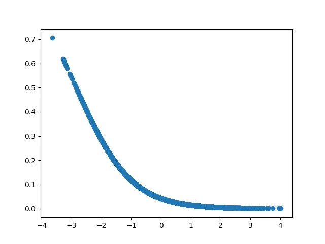
Final layer model: $y = w_1y_1+w_2y_2+w_3+\epsilon_3$
\[w_1 \sim 51.5308, w_2 \sim 91.1138, w_3 \sim -6.4749\]Putting the pieces together, we get the estimate for $y = a_3x^2+b_3x+c_3+\epsilon_4$:
$a_3 \sim 2.9988, b_3 \sim 2.0001, c_3 \sim 0.9998$
Advantage(s) of the bias constrained fit
- The behavior of the fitted function is more predictable over a wider range of data for the weight constrained model compared to the unconstrained model
Drawback(s) of the bias constrained fit
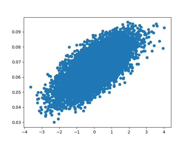
- Given the data there is a high correlation (0.9889) between the two polynomials $y_1$ and $y_2$ — this multi-collinearity may delay convergence, cause the parameter estimates to be unstable. This is much lower for the final layer of the unconstrained model fit: correlation = -0.5862
- The unconstrained fit is closer to the ground truth compared to the constrained fit — in terms of both MSE and coefficients