Unsupervised Exoplanet Detection - from an Autoencoder to a Human-in-the-Loop Pipeline
Introduction
This is a follow-up on the previous article on Unsupervised Exoplanet Detection. Clearly, exoplanet detection is beyond human scale.
I started this project in 2019 with a simple idea: an autoencoder should learn the ordinary behavior of a star, and a poor reconstruction should reveal an anomalous event. A transit is a small, temporary drop in brightness, so it is a natural anomaly for an unsupervised model to find.
The original project used an LSTM autoencoder and interpolation-based preprocessing. It had good recall on the light curves I inspected, but poor precision. Many periodic-looking artifacts were reported as candidates, and the project was limited by CPU training and manual inspection.
I recently returned to the repository. The changes I brought in recently are in response to those limitations. The goal was to make the entire process more reliable: preserve what the telescope actually observed, distinguish useful candidates from artifacts, make results available for review, and turn that review into data for future improvement.
Preserving the signal
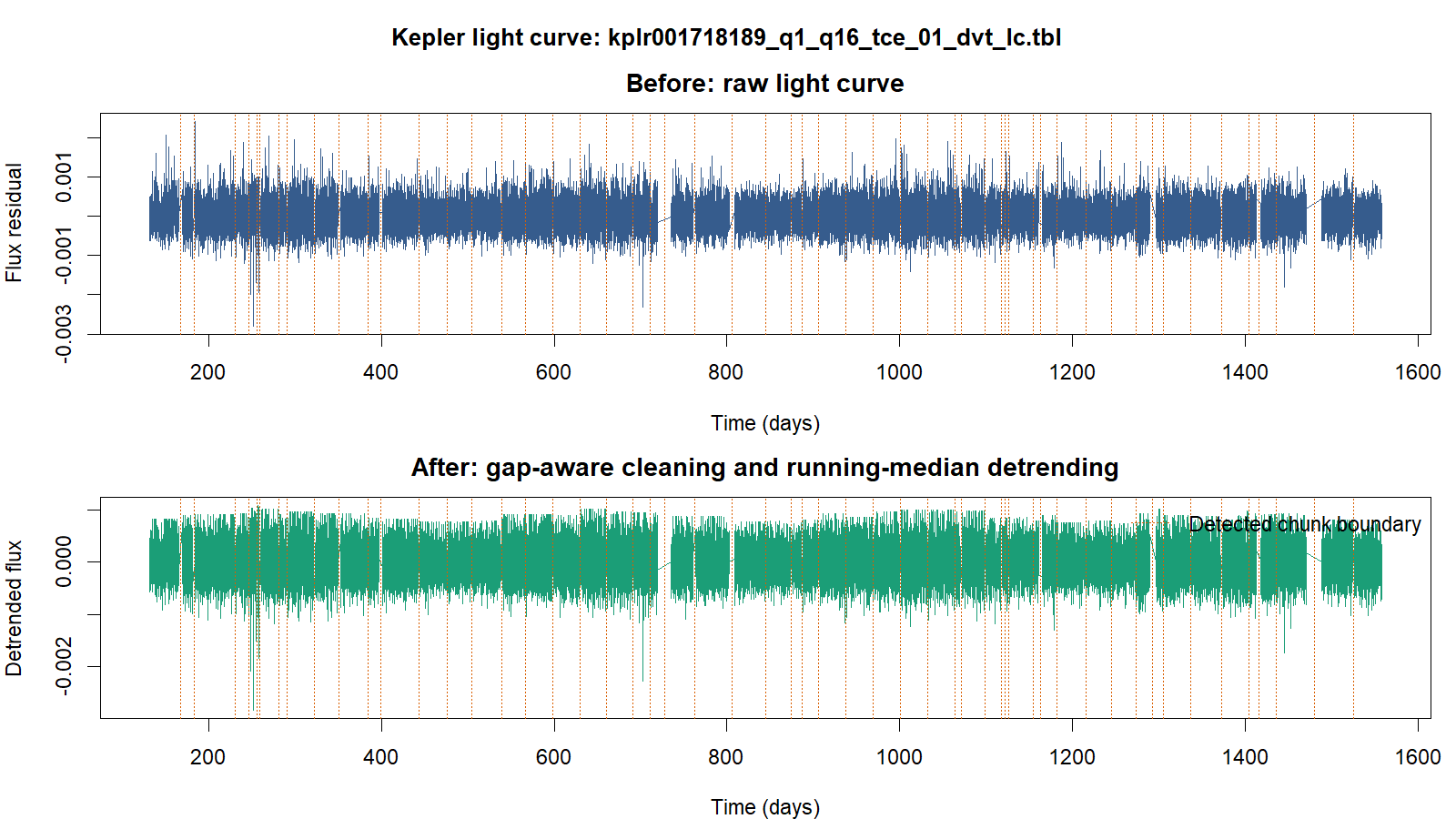
The first problem was preprocessing. Interpolating across a Kepler data gap can create a signal that was never observed. Previously Stineman interpolation was used to fill the gap - this caused unnecessary artifacts (potential false positives). The updated pipeline instead sorts the light curve and splits it into continuous chunks when the time or cadence gap is too large. Fixed-length windows are generated only within those chunks. Each chunk is then detrended with a running median to reduce slow stellar variability. Positive spikes are clipped using a robust MAD-based threshold because flares and cosmic rays are not the negative dips being sought. Negative excursions are retained (transits can only be negative).
Normalization was changed from per-window statistics to one median and MAD computed for each continuous chunk. Per-window normalization can make quiet windows look artificially noisy, while a deep transit can influence the statistics used to measure its own significance. Chunk-level robust statistics provide a more stable estimate of the star’s local noise floor.
These changes address a basic scientific requirement: the detector should not manufacture observations or judge every window against a different definition of ‘normal behavior’.
Making inference practical at scale
The LSTM pipeline was replaced with a one-dimensional convolutional autoencoder. Convolution and pooling compress 128-cadence windows, and upsampling reconstructs them. This structure is suited to local shapes in a time series and can process batches efficiently on a GPU.
Configuration changes
Early stopping and learning-rate reduction were added to the training process. Batch size, sequence length, epochs, paths, and runtime were made configurable. Mixed precision is enabled when a suitable GPU is available and normal float32 execution is available on CPU-only systems. The download and star-parsing code was also moved to native R operations so the pipeline does not depend on a particular shell environment.
The project therefore became easier to run on different machines, but performance was only part of the motivation. A detector that cannot be rerun with explicit settings is difficult to evaluate and improve.
From batch output to review workflow
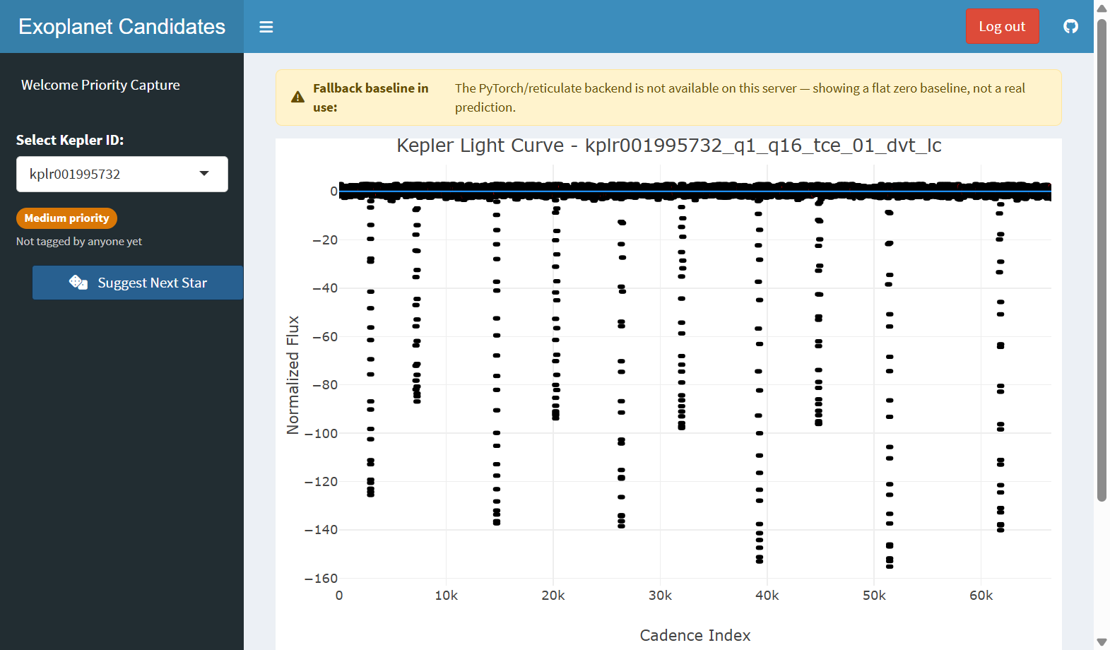
An R Shiny dashboard was already built around the detector. The dashboard reads raw .tbl files on demand, creates and caches plots, loads a star-specific model when available, and falls back to a global model when it is not. When no real model prediction can be produced, the interface shows a reason-specific fallback warning. A zero baseline keeps the application usable, but it should never be mistaken for a model result.
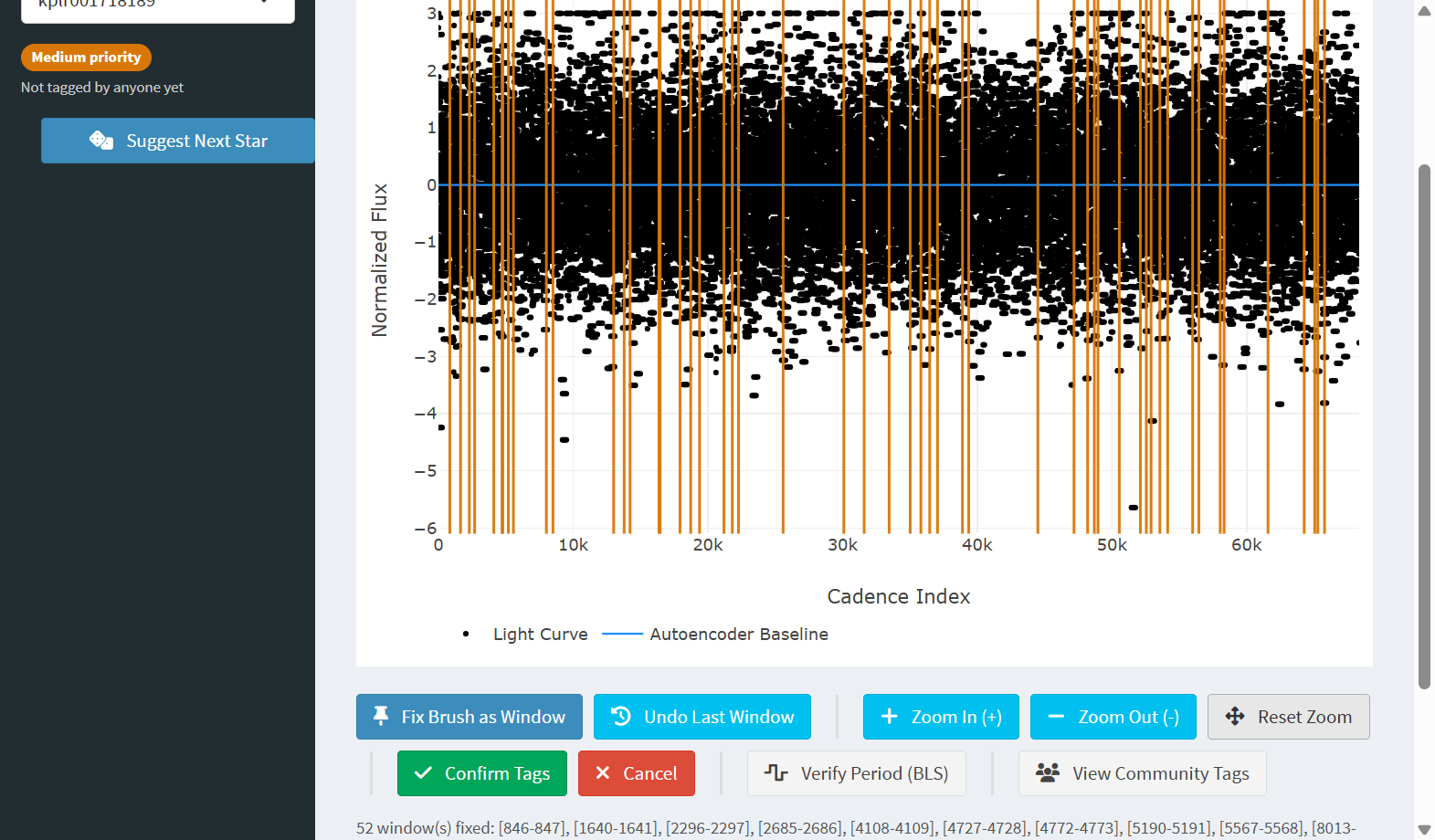
The dashboard alreay supported authentication, session-scoped SQLite connections and zooming. Plotly-based tagging and editable candidate windows were recently added (inspired by Zooniverse -> Planet Hunter TESS). A user can begin with model-generated windows or a blank session, edit the windows, and either confirm or cancel the changes. This is a more useful workflow than treating the model’s indices as final answers.
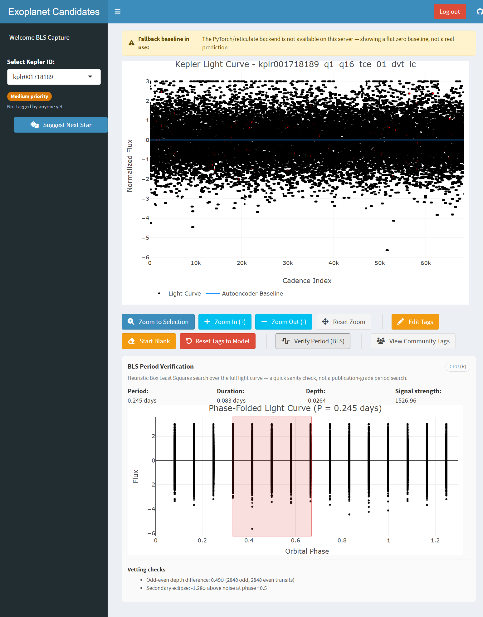
The dashboard also adds astronomy-aware checks after anomaly detection. A Box Least Squares (BLS) search tests whether candidate intervals are consistent with a repeating period. Odd-even depth comparisons and secondary-eclipse checks provide statistical warnings for possible eclipsing binaries or other contaminants. These checks do not establish that a candidate is a planet, but they add information that reconstruction error alone cannot provide.
A Thompson-sampling recommender prioritizes stars based on disagreement between taggers (proposed: human + AI). Stars with no human tags receive an uninformative prior, while overlap between multiple taggers provides a measure of agreement. This makes the review process focus on cases where another human label is most useful. The old unused Stineman interpolation dependency was removed as part of this cleanup to avoid unnecessary artifacts.
Making the system consistent
The project now has a shared scoring path that reads and cleans a star, runs a model-free triage scan, loads the appropriate model, detects candidates, creates plots, and records results. The triage scan deliberately has a high recall. Its purpose is to avoid skipping a potentially real transit before the more expensive model-based analysis runs; false positives are acceptable at this stage. Candidate results are written per star, and a separate script warms the cache offline. This preserves training progress when a long run reaches its time limit or is interrupted.
Still there are practical limits. The force flag signals the models or preprocessing settings to recomputate from scratch. It also prevents duplicate writes without eliminating all repeated inference work. This preserves the state of the past runs and appends new results to the database.
Correctness and human labels
One of the latest fixes addressed the ordering of model outputs. R arrays use column-major ordering, so directly flattening a tensor of windows interleaves points from different windows. That can break contiguous candidate detection, BLS input, plots, and stored indices. The pipeline now explicitly flattens windows in chronological order.
Overlapping windows can also report the same physical transit more than once. Candidate detection now merges nearby detections using the expected overlap between windows (a useful function that can be reused to identify overlap between multiple windows tagged by humans and/or AI).
Human review is now usable as a source of training data. The human tagger groups overlapping user windows into community regions and writes unanimous regions to training_labels_consensus.csv. Partial-agreement regions are written separately to training_labels_disputed.csv. Consensus is not scientific truth, and disagreement is not necessarily an error; disputed regions are useful hard examples for another review pass.
Final words
I started this project as a hobby; I will continue this project as a hobby. Works that started later - such as this article and this paper - are a far more serious undertaking that need considerably more attention than this project.
The current repository is still not a validated exoplanet classifier, it’s an unsupervised ‘anomaly detector’ with some astronomy-aware heuristics such as thresholds, duration limits, BLS search, and vetting rules. A global model improves coverage at the cost of star-specific specialization, and human consensus is an annotation agreement rather than ground truth. Validation/confirmation is still done using slower methods that use powerful telescopes.
The important change is that the project now has a loop: clean the observed data, find unusual behavior, check it against astronomical expectations, let people inspect it, and preserve what they learn for the next iteration.
The long-term goal remains the same: build a system that can identify patterns in astronomical data and reason about why those patterns are credible. The recent changes makes that goal more practical by connecting the model to the scientific and human context required to interpret its predictions. One day I hope to see this pipeline integrated with exoplanet confirmation methods and/or systems.