Ridge Regularization on Linear Regression and Deep Learning Models
Introduction
As discussed in my previous articles on regularization and lasso penalty, regularization can be used to counter overfitting in overparameterized models. Regularization serves as a computationally efficient alternative to best subset selection, but has its disadvantages (Eg: efficiency of the estimator is low). The objective of this article is to introduce the mathematical basis of ridge regression, derive its analytical solution, discuss its geometric interpretation and relate it to SVD for component-wise analysis.
Formulation
Formulation and normal equation form of linear regression can be found in my previous article.
Ridge formulation and solution
\[Y=X\beta + \epsilon \tag{Linear Regression}\] \[y=x\hat\beta^{(Ridge)} + \hat{e}^{(Ridge)} \tag{Ridge solution estimated on a sample}\] \[L=||y-x\beta||_2^2 + \lambda||\beta||_2^2=(y-x\beta)^T(y-x\beta) + \lambda \beta^T \beta \tag{Ridge loss function}\] \[\hat\beta^{(Ridge)}=argmin_{\beta}L = argmin_{\beta}[(y-x\beta)^T(y-x\beta) + \lambda \beta^T \beta] \tag{Ridge solution}\] \[\frac{\partial L}{\partial \beta}|_{\beta=\hat\beta^{(Ridge)}}=0 \implies 2[-x^T(y-x\hat\beta^{(Ridge)})+\lambda\hat\beta^{(Ridge)}]=0 \implies \hat\beta^{(Ridge)}=(x^Tx+\lambda I)^{-1}x^Ty \tag{Ridge estimate using normal equation}\]Note: Ridge can be viewed as a penalty that modifies the covariance matrix, thereby reducing collinearity between the variables. This property of ridge helps in avoiding plateaus in the loss function.
Geometric interpretation
Dual form of optimization
\[L(\beta) = ||y-x\beta||_2^2 + \lambda ||\beta||_2^2 \tag{Primal form of ridge optimization (unconstrained)}\] \[min(L(\beta)) \sim min(||y-x\beta||_2^2) s.t. ||\beta||_2^2 \le s; s=f(\lambda) \tag{Dual form of ridge optimization (constrained)}\]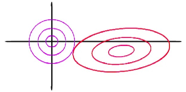
The purple circles correspond to $|\beta|_2^2 \le s$ for different $s$, where $|\beta|_2^2 = constant$ along a circle. Increasing $\lambda$ decreases the size of the circle by decreasing $s$. The red ellipses correspond to different distinct values of $||y-x\beta||_2^2$ where $||y-x\beta||_2^2 = constant$ along an ellipse. For a fixed $\lambda$ the value of $s$ is fixed: this corresponds to one of the purple circles.
The minimum value of $||y-x\beta||_2^2$ in unconstrained case occurs at the center of the ellipse. However, under the constrained case of $|\beta|_2^2 \le s$ the solution will be displaced towards the origin.
The unique ridge solution is located at the point where these two ‘curves’ touch. Since the curve $|\beta|_2^2 \le s$ is differentiable throughout, the ridge solution for all $\beta$s will be non-zero for finite $\lambda$. On increasing $\lambda$ (decreasing $s$) the $\beta$s are moved closer to 0. This does not causes sparsity for finite $\lambda$ even though the $\beta$s are moved closer to 0. Therefore, ridge penalty cannot be used for feature selection.
Relating ridge penalty and SVD (PCA)
Applying SVD on x, we get $x=UDV^T$. Substituting this in the analytical solution of ridge, assuming the independent variables are centered and using the properties of rotation and projection matrices we get
\[\hat{\beta}^{(Ridge)}=(VD^TU^TUDV^T+\lambda VV^T)^{-1}VD^TU^T y=(V[D^TD + \lambda I]V^T)^{-1}VD^TU^T y\] \[\implies \hat{\beta}^{(Ridge)}=(V^T)^{-1}(D^D+\lambda I)^{-1}V{-1}VD^TTU^T y=V(D_2+\lambda I)^{-1}D^TU^T y \tag{Ridge solution in terms of principal components}\] \[\hat{y}^{(Ridge)}=x\hat{\beta}^{(Ridge)}=UDV^TV(D_2+\lambda I)^{-1}D^TU^T y=UD(D_2+\lambda I)^{-1}D^TU^Ty=UD_{2,1}U^Ty \tag{Ridge prediction}\] \[D_{2,1}[i]=\frac{D^2[i]}{D^2[i]+\lambda} \tag{Diagonal matrix in ridge prediction}\] \[\hat{y}^{(Ridge)}=\sum_{i=1}^{p}U_i\frac{d_i^2}{d_i^2+\lambda}U_i^T y \tag{Ridge prediction}\]Let us examine this step-by-step:
- Project $y$ in the space of $PC_i$, where $PC_i$ refers to the $i^{th}$ principal component. All projections will be in the column space of $x$
- Scale down the projection by a factor (strict scale down happens for $\lambda > 0$)
- Re-transform the projection
From the above equation we can approximate the degrees of freedom of a regression model penalized using ridge as $df_{Ridge} = \sum_{i=1}^{p}\frac{d_i^2}{d_i^2+\lambda}$
Extension to deep learning
Deep learning suffers from overfitting when the weights at a particular layer are correlated. This usually happens in the fully-connected part of the network. Ridge projects the output feature map of the training set on the principal components and shrinks the prediction. This makes the loss curve more convex even in cases of perfect collinearity between independent variables. For a suitably chosen $\lambda$ the weights will be very small. Therefore, in presence of ridge penalty the non-linearity builds up slowly as we perform a forward pass through the network. This argument also applies to small $\lambda$.
Conclusion
In the previous article we discussed lasso regularization as a way of tackling overfitting by performing variable selection. Ridge regression is useful when feature elimination needs to be forcibly suppressed. In real-life problems this property is useful when the exhaustive set of features is known and all features are of ‘scientific value’ to the outcome: therefore no feature can be dropped from the analysis. However, when prediction accuracy is of importance, a linear combination of lasso and ridge penalties is used. This is called elasticnet. The proportion of L1 regularization is also a hyperparameter that should be tuned along with other hyperparameters. Elasticnet is a general case of L1 and L2 regularization. It is expected to outperform ridge and lasso when tuned appropriately on the validation set.
\[\frac{1-\alpha}{2}||\beta||_2^2 + \alpha ||\beta||_1 \tag{Elasticnet. Equation credit: glmnet package documentation}\]