Extending the house-hunting agent - adding datasets without adding code
In my last post I listed what was still missing from the new app - crime, walkability, flood boundaries, more sold-home coverage - and closed by saying each new source could just be “Clauded” and added to the respective prompts as needed. In this article I will describe how data on crime and bike infrastructure were added to the data ingestion layer, to the dashboard layer and to the ‘General Chat’ agent. I will conclude by showing how to add other new data to the app.
What actually changed
The metadata catalog
The list of possible tables and joins/relationships was previously defined in the system prompt (independent of the query). This bloated the prompt - the ‘agent’ was using an extremely long prompt to reason about simple questions; this may cause context rot and lead to inconsistent answers from the agent. Now, db/schema_catalog.py abstracts out the information about tables and joins — which tables exist, which columns are reliable vs. noisy, which joins are valid, what filters and caveats matter. As a result, the agent reads only the information about necessary tables and joins based on the input query at runtime.
The data/app layer
The following changes were made to the data/app layer:
db/duckdb_store.pyis a cleaner abstraction over the actual database instead of connection and query code scattered across services.- New loaders were added to
services/data_loader.py- one for each new dataset (crime, bike infrastructure).- One parser per city for crime defined in
services/crime_sources.py- as seen in the previous app, crime data is heterogeneous across cities. These parsers harmonize incident data into a common taxonomy. - A parser for bike infrastructure - bike infrastructure data may also be heterogeneous across cities.
- One parser per city for crime defined in
- Map layers were added to
services/layers.py- NRI (existing data, new layer), crime (new), bike infrastructure (new).
New specialized tools were written only for complex segments - Eg: segments that cannot be SQLized. For example, a Dijkstra’s shortest path tool was added for the bike infrastructure dataset to look for ‘safe’ bike routes between two locations that are passed to the agent. None of this touches the stack from last time - same FastAPI backend, same two LangGraph agents, same DuckDB and ChromaDB - core architecture remains the same. Only the prompt was cleaned up as described in the metadata catalog section.
The only hard dependency
Redfin lets you export your favorites as a CSV with address, lat-lon, price, square footage and a few other fields for free. Currently this app has a hard dependency on Redfin’s favorites. However, I’ll work on removing that dependency in the future - all that’s needed is the address; geocoding and walkscore (see R code from the previous app) APIs will be called on the fly; I’m yet to decide on a way to ingest price, sqft, etc.
This app is close to a blank canvas: it works off bare minimum data about houses, “Claudes” one dataset at a time and “Claudes” one tool at a time. Complex questions are offloaded to the LLM/agent’s “planning” phase.
Wiring up the new datasets with the agent
The current agent design gets rid of dataset-specific tools and prompts. Here’s an example in action: once the standardized crime table exists and is added to schema_catalog.py (what it joins to, on what key, what the taxonomy column means), the agent doesn’t need a crime-specific tool. get_database_schema fetches the new table name for the agent’s planning phase; query_database uses the schema and relationships to build the query (using the LLM). No more “if the user asks about crime” prompt branch!
Ingesting and harmonizing bike routes is a one-time plumbing activity - same as crime. But routing over the bike network - actually finding a path across a graph of facilities - isn’t a simple ‘SQL join’. It may be difficult for the LLM/agent to produce the necessary code - so ‘bike routing’ got its own tool.
Note: if the answer can be derived from ‘relations’ in the ‘relational data’, schema_catalog.py plus query_database can handle it with no new code. If the answer requires an algorithm - a route, a distance calculation, etc. - it needs a new tool. Crime turned out to be the first kind. ‘Safe’ bike routing is the second.
Adding new datasets - the same recipe
Different people have different needs. Walkability and ‘safe’ drinking water were a few of my needs. EPA’s Smart Location Database - neighborhood-scale walkability built on Census block-group geography and lead service line / water infrastructure data need to be added to meet my goal.
The recipe is the same - the new data can be ‘Clauded’ as shown below:
- Add the table to
db/duckdb_store.py. - Add the join logic to
db/schema_catalog.py- Eg: walkability links to the same tract/block-group geometry as NRI and census; lead line links using parcel or address (services/geocoder.py, the pipeline built for sold-home comps, also solves the same problem). - Add a loader in
services/data_loader.py, flag the data’s actual granularity - parcel-level vs. service-area estimate - as a caveat in the catalog. - Let the agent discover it. No new tool. No new prompt branch. No “walkability question” or “lead pipe question” handler.
What’s interesting is that the moment both tables and their join keys exist in schema_catalog.py, they sit in the same reasoning space as crime, bike infrastructure, NRI, sold-home comps, and census/CBSA context that are already available. Nobody has to write a tool for the combination because the LLM/agent reasons using the schema and relationships!
However, a new tool is needed if a complex algorithm is required to infer the answer from the data. For example, if a public transit network + timing data and a specialized ‘planning tool’ are available the agent can make a public transit plan between two locations by finding a path over the transit network (shortest path/time depending on the need).
Concretely: once those two tables exist, a question like “which of my favorites are in the top quartile for walkability, have no known lead service line risk, and sit in a tract with below-average crime over the last year” (query_database uses the LLM/agent’s reasoning to identify the joins across four tables to answer this question; no new tool needed) becomes answerable with zero new Python!
The actual advantage
The design was not a coincidence. Adding new data to my old app was a challenging task - hand-coding new data loaders and new story-driven layers took time (this was before the LLM coding era). The ‘code agent’ approach from the last post (get_database_schema and query_database in place of a tool per question) was a deliberate design choice made specifically so both the ingestion layer and the agent layer could grow without hardcoding or one-off workflows for each new data source. A new dataset only needs a loader and a catalog entry, not a new tool or a new prompt branch. This is the same “metadata in, code out” idea from the previous post, just proven on a harder case and scaled up for more complex scenarios.
The per-house agent’s five tools (comps math, the NRI lookup, and the rest) are still hand-written and not schema-driven - this is a problem for another day.
A real example to top it all off
Visuals:
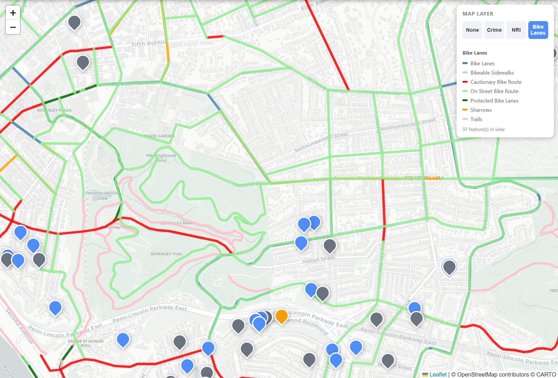
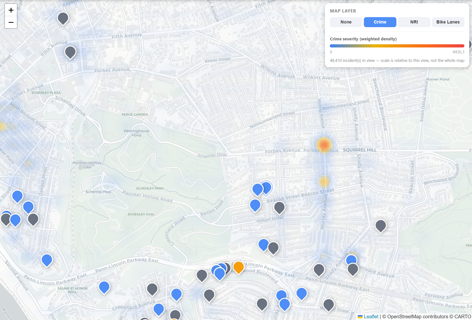
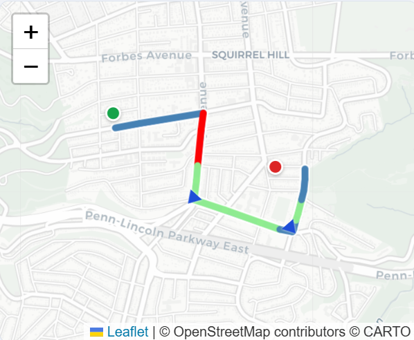
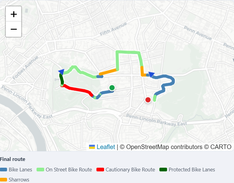
Question to the agent: Find the shortest bike route from 5534 Raleigh St, Squirrel Hill, PA 15217 to 6324 Waldron St, Pittsburgh, PA 15217
Yes — a continuous BikePGH route was found.
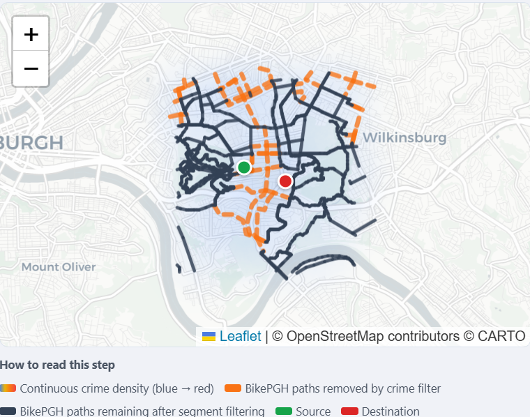
Question to the agent: Find a bike route from 5534 Raleigh St, Squirrel Hill, PA 15217 to 6324 Waldron St, Pittsburgh, PA 15217 that avoids some of the crime prone areas in Pittsburgh.
Yes — a continuous BikePGH route exists after filtering out the selected high-density crime areas.
Intermediate: crime filter applied to BikePGH top 10% density cells excluded 21 hotspot cells shown 3,532 BikePGH edges removed 1,580 network segments shown Crime density is shown as a continuous heatmap using the same normalized score that drives routing. When a logical BikePGH segment between two junctions intersects a buffered top-percentile crime hotspot, the entire segment is removed; clean segments remain unfiltered.
Final bike route 4.7 mi · 28 min estimate
Pending
- National Walkability Index
- Raw polygons for lead pipes
- FEMA’s actual flood hazard polygons
- Zillow’s home value and market heat indices
- Sold-home county parsers for additional counties
- Converting the per-house agent to the same schema-driven path as general chat
Code’s on GitHub. Same closing note as last time: none of this replaces an actual realtor, an actual inspection or actually walking the block at 7pm on a Tuesday. It just means better and more relevant data, better inferences, better decisions.